Tutorial
This tutorial will go through all the functionality in FeynSimul. First
Import FeynSimul and a physical system
This imports the kernel module that contains the class PIMCKernel class that is the heart of the computations. The kernel_args module contains an empty classed called kernelArgs which is used to hold the arguments to the PIMCKernel class. A physical system is also imported. In this case this is a simple harmonic oscillator, that is a particle in a \(V(x) = kx/2\) potential.
>>> from FeynSimul.kernel import PIMCKernel
>>> from FeynSimul.kernel_args import KernelArgs
>>> from FeynSimul.physical_systems.harm_osc import HarmOsc
Setting the parameters in a run
What we first do is create an instance of the KernelArgs which will hold the parameters for the simulation. This class does not contain any methods and is just for convenience. The class initiatior contains quite a lot of parameters and what these do and which ones are needed to define can be read about in the documentation for KernelArgs.
>>> phys_system = HarmOsc()
>>> ka = KernelArgs(system = phys_system,
                    nbrOfWalkers = 32 * 28,
                    N = 128,
                    beta = 11.0,
                    S = 6,
                    enableOperator = True,
                    enableCorrelator = False,
                    metroStepsPerOperatorRun = 40,
                    enableBisection = True,
                    enablePathShift = False,
                    enableSingleNodeMove = False,
                    enableParallelizePath = True,
                    enableGlobalPath = False,
                    enableGlobalOldPath = False,
                    enableBins = False,
                    operatorRuns = 150,
                    nbrOfWalkersPerWorkGroup = 4,
                    operators = (phys_system.energyOp,))
When the kernel parameters are set the PIMCKernel class can be created with the KernelArgs instance as argument.
>>> kernel = PIMCKernel(ka)
Running the kernel and retrieving values
To run the simulation one simple uses the run method in the PIMCkernel object.
>>> kernel.run()
We can now fetch the mean of the operators for each independent simulation and calculate for example the mean of them using numpy.
>>> import numpy as np
>>> operatorValues = kernel.getOperators()
>>> print np.mean(operatorValues)
0.499803373124
This is fairly close to the analytical result 0.5.
Calculating the probability density
If we want the calculations to include the probability density of the particle in its ground state we need to enable it and rebuild the kernel with the updated settings
>>> ka.enableBins = True
Some parameters need to be set when the kernel is run with enableBins active. These determines what interval to calculate the density function in and how fine resolution should be used. Points outside the interval will be discarded.
>>> ka.xMin = -3.5
>>> ka.xMax = 3.5
>>> ka.binResolutionPerDOF = 80
Now after we recreate the PIMCkernel object to update it with the new setttings and run it, the probability density can be fetched.
>>> kernel = PIMCKernel(ka)
>>> kernel.run()
>>> probDensity = kernel.getBinCounts()
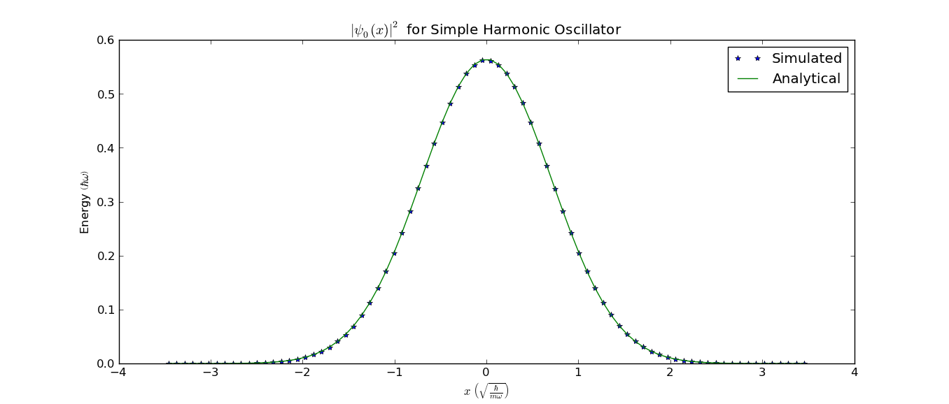
We could now plot it and compare it with the analytical solution:
>>> import pylab as pl
>>> binSize = (ka.xMax - ka.xMin) / ka.binResolutionPerDOF
>>> x = np.linspace(ka.xMin, ka.xMax - binSize,
            ka.binResolutionPerDOF) + 0.5 * binSize
>>> pl.plot(x, probDensity, '*', label="Simulated")
>>> pl.plot(x, 1/np.sqrt(np.pi) * np.exp(-x ** 2), label="Analytical")
>>> pl.legend(loc="best")
>>> pl.show()
This would give this figure (without the labels) where the calculated and analytical result agree well:
Using correlator function to get excited energy state
We can get the energy for the first excited state by exploiting calculating the autocorrelation of the values of the nodes in the path. Enabling the correlator calculation will calculate the autocorrelation for lags up to N / 2.
>>> ka.enableCorrelator = True
>>> ka.correlators = ("x1",)
>>> kernel = PIMCKernel(ka)
>>> kernel.run()
We can now get the correlation like with the probability density. getCorrelator returns a tuple with the correlator means and the standard error. For now we are only interested in the means so we extract the first index.
>>> corrs = kernel.getCorrelator()[0]
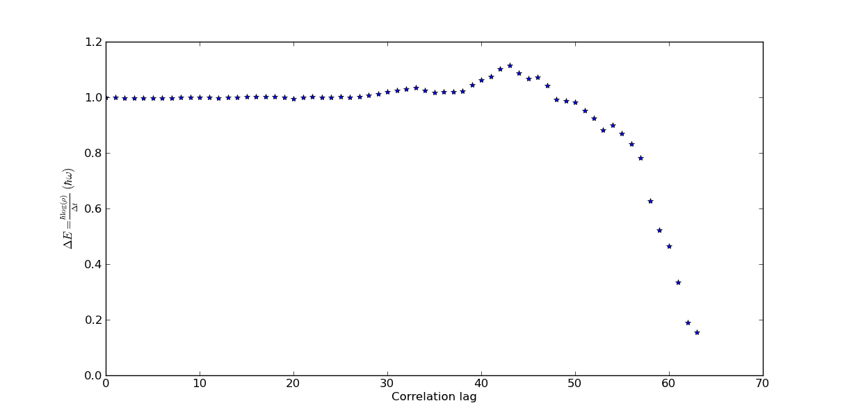
The negative log derivative of the correlation gives the difference in energy between the ground state and first excited state. We can plot this
>>> import pylab as pl
>>> logDerCorr = -np.gradient(np.log(corrs[0]), ka.beta / ka.N)
>>> pl.plot(logDerCorr, '*')
>>> pl.show()
This would give the following figure (without labels) in which we can read that the difference in energies are about \(1.0 \hbar \omega\) which is correct.
The modN function
This is a function made to help with some common things one would like to do like saving data, resuming an earlier simulation etc. To read more about the arguments to the function and what it does you can read the PimcUtils documentation.
In this tutorial we will once again use the simple harmonic oscillator system. A small run will be done to see how the function works. To start off we import the function together with the system as well as the class that will hold our arguments.
>>> from FeynSimul.pimc_utils import modN
>>> from FeynSimul.kernel_args import KernelArgs
>>> from FeynSimul.physical_systems.harm_osc import HarmOsc
As before we make an instance of the KernelArgs class. Since the function only works with the bisection sampling method we enable it. This is basically the same thing as earlier.
>>> ka = KernelArgs(nbrOfWalkers = 448,
                    N = 8,
                    enablePathShift = False,
                    enableBisection = True,
                    enableSingleNodeMove = False,
                    enableGlobalPath = True,
                    enableGlobalOldPath = True,
                    enableParallelizePath = True,
                    enableBins = False,
                    beta = 20.0,
                    nbrOfWalkersPerWorkGroup = 4,
                    operatorRuns = 300,
                    enableOperator = True,
                    enableCorrelator = False,
                    metroStepsPerOperatorRun = 40,
                    system = HarmOsc(),
                    operators = (HarmOsc.energyOp,))
We then specify some of the arguments to use in the modN function.
First we set the total time in seconds to run the simulation.
>>> endTime = 10
Then we set how frequently to save paths.
>>> savePathsInterval = 30
Each initial path is s straight line in space. One argument to the function is an array where each index determines where Here we make each path start of in a random interval between -0.01 and 0.01.
>>> import numpy as np
>>> startPaths = np.random.uniform(size=(ka.nbrOfWalkers,ka.system.DOF),
                                   low=-1.0, high=1.0) * 0.01
We then have to define how different parameters should scale with N and S.
>>> def opRunsFormula(N, S):
        return max(2 ** 10 / 2 ** S, 1)
>>> def mStepsPerOPRun(N, S):
        return 10
>>> def runsPerN(N, S):
        return max(N / 8, 8)
We can now start the function
>>> modN(ka, startPaths, savePathsInterval, "SHO", opRunsFormula,
         mStepsPerOPRun,  runsPerN, 512, simTime=endTime, finalN=256,
         verbose=True)
This would give output similar to the following. We can see that when N goes from 8 to 16 the value of the operator changes substantially. At higher N this change becomes very small and we can then said to have an N large enough. Of course in real run better analysis should be done.
>>> New kernel compiled, getStats():
    Global memory (used/max): 592 B / 1.02e+03 MiB
    Local memory (used/max): 0 B / 48 kiB
    Workgroup size (used/device max/kernel max): 16 / 1024 / 960
    Workgroup dimensions (used/max): (4, 4) / [1024, 1024, 64]
    Number of workgroups (used): 1
    Run results:
    N: 8    S: 1    beta: 20.0      AR: 0.556884765625      OPs: [ 0.31128057]
    N: 8    S: 1    beta: 20.0      AR: 0.56064453125       OPs: [ 0.3144856]
    N: 8    S: 1    beta: 20.0      AR: 0.561181640625      OPs: [ 0.31377281]
    .
    .
    .
    N: 16   S: 2    beta: 20.0      AR: 0.4765625           OPs: [ 0.42442046]
    N: 16   S: 2    beta: 20.0      AR: 0.479248046875      OPs: [ 0.42519391]
    N: 16   S: 2    beta: 20.0      AR: 0.474145507812      OPs: [ 0.41078902]
    N: 16   S: 2    beta: 20.0      AR: 0.476831054687      OPs: [ 0.42454475]
    N: 16   S: 2    beta: 20.0      AR: 0.47412109375       OPs: [ 0.42009237]
    .
    .
    .
    N: 64   S: 2    beta: 20.0      AR: 0.892547607422      OPs: [ 0.49482867]
    N: 64   S: 2    beta: 20.0      AR: 0.892272949219      OPs: [ 0.49900044]
    N: 64   S: 2    beta: 20.0      AR: 0.892462158203      OPs: [ 0.48953001]
    N: 64   S: 2    beta: 20.0      AR: 0.893359375         OPs: [ 0.496154]
    .
    .
    .
A datafile is also saved and from it we could create a plot such as the one below. Here it can clearly be seen how the differences in the energy when increasing N become smaller as N becomes larger.